Diagonalising 2D Schrödinger Equation
The text and method is based on the following sources:
- Youtube, 2D Schrodinger Equation Numerical Solution in PYTHON, (2022), Available at: (Accessed: 6 March 2022).
- Alexvas, Discretization of Laplacian with boundary conditions, (2017), Available at: (Accessed: 6 March 2022).
- Thomas H. Pulliam, David W. Zingg., Fundamental Algorithms in Computational Fluid Dynamics, (2014), Springer.
1using PyPlot, PyCall
2using LinearAlgebra
3using SparseArrays
4using Arpack, KrylovKit
Two-dimensional box
The goal is to solve the single particle Schrödinger equation in a two-dimensional box of length $2L$ of the Hamiltonian: $$ \hat{h}=\frac{-\hbar^{2}}{2 m} \nabla^{2}+V(\mathbf{r}, t). $$ The box can have a homogeneous Dirichlet boundary condition, i.e., the wave function evaluated at the border must vanish, or periodic boundary conditions. There can be a potential $V$ in the box. So let us a meshgrid of $\mathbf{x}$ and $\mathbf{y}$ coordinates.
 1N = 100
 2L = 10.0
 3Δx² = (2*L/N)^2
 4function meshgrid(x, y)
 5    X = [x for _ in y, x in x]
 6    Y = [y for y in y, _ in x]
 7    X, Y
 8end
 9x = LinRange(-L, L, N)
10y = LinRange(-L, L, N)
11X, Y = meshgrid(x, y);
Potential
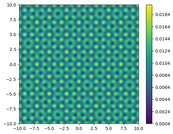
The potential is chosen to be eightfold rotation symmetric quasicrystal, centered on $\mathbf{r}=0,$ $$ V(\mathbf{r})=V_{0} \sum_{k=1}^{4} \cos ^{2} \left(\mathbf{G}^k \cdot \mathbf{r}\right), $$ where $V_{0}$ is the potential amplitude and the quantities $G^{k}$ are the lattice vectors of four mutually incoherent standing waves oriented at the angles $0^{\circ}, 45^{\circ}, 90^{\circ}$, and $135^{\circ}$, respectively. The lattice vectors have norm $\left|G^{k}\right|=\pi / a$.
1function get_potential(x, y, V₀)
2    return V₀*(cos(pi*x)^2 + cos(pi*√2/2*(x+y))^2 + cos(pi*y)^2 + cos(-pi/(√2)*(x-y))^2)
3end
4
5V = get_potential.(X,Y, 0.005)
6fig = figure(figsize=(6.2,5))
7contourf(X, Y, V, 50)
8colorbar()
Units
The Schrödinger equation is given by $$ \left[\frac{-\hbar^{2}}{2 m} \nabla^{2}+V(\mathbf{r})\right] \psi(\mathbf{r}) = E\psi(\mathbf{r}),$$ Let us use the lattice spacing $a$ and the corresponding recoil energy $E_r = \pi^2\hbar^2/2ma^2$ as the space and energy units, respectively, such that we have
$$ \left[\frac{-\hbar^2}{2 m E_ra^2} \tilde{\nabla}^{2}+\frac{V(\mathbf{\tilde{r}})}{E_r}\right] \psi(\mathbf{\tilde{r}}) = \left[ \frac{-1}{\pi^2} \tilde{\nabla}^{2}+\tilde{V}_{0} \sum^4_k \cos^{2}\left(\tilde{\mathbf{G}}^{k} \cdot \tilde{\mathbf{r}}\right) \right] \psi(\mathbf{\tilde{r}}) = \tilde{E}\psi(\mathbf{\tilde{r}}), $$
where $|\tilde{\mathbf{G}}_{k}|=\pi$, $\tilde{\mathbf{r}} = \frac{\mathbf{r}}{a}$, and $\tilde{E}=\frac{E}{E_r}$.
Discretize in one dimension
Rest us to discretize our Hamiltonian. The idea can be easily explained by the following finite difference approximation of the second derivative in one dimension $$ \frac{d^2 \psi}{dx^2} \approx \frac{\psi_{i+1}-2\psi_i + \psi_{i-1}}{\Delta x^2}.$$
Dirichlet boundary conditions
Suppose we have $M=4$ interior points and $a$ and $b$ two boundary points, a mesh with four interior points $\Delta x=2L /(M+1)$, represented as follows $$ \begin{aligned} &\qquad \ \ \ \ a \ \ \ 1 \ \ \ 2 \ \ \ 3 \ \ \ 4 \ \ \ b \\\ &x=- \ L \ - \ - \ - \ - \ \ L \end{aligned} $$ We impose Dirichlet boundary conditions, $u(-L)=u_{a}, u(L)=u_{b}$ and use the centered finite difference approximation at every point in the mesh. We arrive at the four equations:
$$ \left(d_{x x} u\right)_{1} =\frac{1}{\Delta x^{2}} (u_a - 2 u_1 + u_2) $$
$$ \left(d_{x x} u\right)_{2} =\frac{1}{\Delta x^{2}} (u_1-2 u_2+u_3) $$
$$ \left(d_{x x} u\right)_{2} =\frac{1}{\Delta x^{2}} (u_2-2 u_3+u_4) $$
$$ \left(d_{x x} u\right)_{4} =\frac{1}{\Delta x^{2}}\left(u_3-2 u_4+u_b\right) $$
Introducing $$ \begin{aligned} \vec{u}=\left( \begin{array}{c} \psi_{1} \\\ \psi_{2} \\\ \psi_{3} \\\ \psi_{4} \end{array} \right) \quad (\overrightarrow{b c})=\frac{1}{\Delta x^{2}} \left( \begin{array}{c} \psi_{a} \\\ 0 \\\ 0 \\\ \psi_{b} \end{array} \right) \quad A=\frac{1}{\Delta x^{2}} \left( \begin{array}{rrrr} -2 & 1 & & \\\ 1 & -2 & 1 & \\\ & 1 & -2 & 1 \\\ & & 1 & -2 \end{array} \right) \end{aligned} $$ we can rewrite in matrix form as $$ \begin{aligned} \frac{d^2 \psi}{dx^2} =\frac{1}{\Delta x^{2}}D= A \vec{\psi}+(\overrightarrow{b c}) \end{aligned} $$
Periodic boundary conditions
This subsection has to be tested and worked out. First try did not work.
Suppose we have $M=8$ points on a linear periodic mesh, represented as follows $$ \begin{aligned} &\cdots \ \ \ 7 \ \ \ \ 8 \ \ \ \ \ \ a \ \ \ \ 1 \ \ \ \ 2 \ \ \ \ 3 \ \ \ \ 4 \ \ \ \ b \ \ \ \ 1 \ \ \ \ 2 \ \ \ \cdots \\\ &x= \ - \ \ - \ \ -L \ \ - \ \ - \ \ - \ \ - \ \ L \ \ - \ \ - \end{aligned} $$ where we have that $\psi(L)=\psi(-L)$. It can be shown that the matrix representation is modified by $$ \begin{aligned} \frac{d^2 \psi}{dx^2} =\frac{1}{\Delta x^{2}}D_p=\frac{1}{\Delta x^{2}} \left( \begin{array}{rrrr} -2 & 1 & & 1 \\\ 1 & -2 & 1 & \\\ & 1 & -2 & 1 \\\ 1 & & 1 & -2 \end{array} \right) \end{aligned} $$
Discretize in two dimensions
In two dimensions, the wavefunction is not a vector anymore but a matrix. However, we would like to write it back as vector via the transformation $$ \left( \begin{array}{rrrr} \psi_{11} & \psi_{12} & \cdots & \psi_{1N} \\\ \psi_{21} & \psi_{22} & \cdots & \psi_{2N} \\\ \vdots & \vdots & \ddots & \vdots \\\ \psi_{N1} & \psi_{N2} & \cdots & \psi_{NN} \end{array} \right) \rightarrow \left( \begin{array}{c} \psi_{11} \\\ \psi_{12} \\\ \vdots \\\ \psi_{NN} \end{array} \right) $$ The second derivative finite difference matrix must than be written as $$ \frac{\partial^2 \psi}{\partial x^2} = \frac{1}{\Delta x^{2}} I \otimes D = \frac{1}{\Delta x^{2}} \left( \begin{array}{rrr} D & & \\\ & \ddots & \\\ & & D\end{array} \right) $$ where $\otimes$ is the Kronecker product. The 2D Laplacian can than be written as $$ \nabla^{2} = \frac{\partial^2 \psi}{\partial x^2} + \frac{\partial^2 \psi}{\partial y^2} = \frac{1}{\Delta x^{2}} (I \otimes D + D \otimes I) = \frac{1}{\Delta x^{2}} D\oplus D $$ where $\oplus$ is the Kronecker sum, and we used that we discretized space as a squared grid, i.e. $\Delta x^{2}=\Delta y^{2}$.
Hamiltonian
Let us assume the homogeneous Dirichlet Boundary conditions $\psi(L, y) = \psi(-L, y) = \psi(x, L) = \psi(x, -L) = 0$. The discretized Schrödinger equation can then be written as
$$
\left[-\frac{1}{\pi^2}(D \oplus D) + \Delta x^2 \tilde{V} \right] \psi = \left( \Delta x^2 \tilde{E}\right) \psi,
$$
where $D$ has -2 on the main diagonal and 1 on the two neighboring diagonals and $\psi$ is a vector. One could define the potential in units of $\Delta x^2$; in other words get_potential actually returns $\Delta x^2 V$. However, we will leave $\Delta x^2$ in the kinetic term.
Now we construct
$$
\hat{h} = -\frac{1}{\Delta x^{2}\pi^2} D \oplus D + \tilde{V}
$$
such that the corresponding eigenvalues $\tilde{E}$ are in units of recoil energy $E_r$.
Let $T=-\frac{1}{\Delta x^{2}\pi^2} D \oplus D$ and $U = V$
1diag = ones(N); # vector of ones
2diags = Vector([diag[begin:end-1], -2*diag, diag[begin:end-1]]); # vector of vectors of the diagonals
3D = sparse(Tridiagonal(diags...)) # creates the discretised 2nd derivative
4T = -1/(Δx²*pi^2) * (kron(D, sparse(I,N,N)) + kron(sparse(I,N,N), D))  #N**2 x N**2 matrix
5U = spdiagm(reshape(V, N^2))
6H = T+U;
Here we used the package SparseArrays.jl to make the computations faster. Sparse arrays are arrays that contain enough zeros that storing them in a special data structure leads to savings in space and execution time, compared to dense arrays.
Eigenvectors and eigenvalues
Now that we constructed our discretized Hamiltonian we can just exactly diagonalize our Hamiltonian to find the eigenvalues and eigenvector. We shall to this with the package Arpack.jl which is a Julia wrapper to a FORTRAN 77 library designed to compute a few eigenvalues and corresponding eigenvectors of large sparse or structured matrices, using the Implicitly Restarted Arnoldi Method (IRAM) or, in the case of symmetric matrices, the corresponding variant of the Lanczos algorithm. Both are classified as Krylov subspace based algorithms (see wikipedia). It is used by many popular numerical computing environments such as SciPy, Mathematica, GNU Octave and MATLAB to provide this functionality.
We use the eigs function where nev specifies how many eigenvalues and eigenvectors we want and which specifies the type of eigenvalues to compute. For my purposes I only need the ground state wave function.
Alternatively, one could use KrylovKit.jl, a native Julia package collecting a number of Krylov-based algorithms for linear problems, singular value and eigenvalue problems and the application of functions of linear maps or operators to vectors. With KrylovKit.jl I manage to find better results if when I increase the number of point $N$. My theory is that it, as black box solver, uses another method above a certain threshold $N^*$, whereas Arpack.jl sticks to the same method and hence gives worse results.
1# eigenvalues, eigenvectors = eigs(H, nev=1, which=:SM);
2_, vecs, _ = eigsolve(H, 1, :SR);
3# vecs[1]
As we constructed the Hamiltonian to be a $N^2 \times N^2$ so that $\psi$ could be a vector, we have to reshape the eigenvectors back to a $N \times N$ matrix.
1function get_e(n::Int64)
2    return reshape(vecs[1]', N, N)
3end;
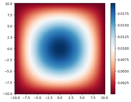
1figure(figsize=(6.2,5))
2pcolormesh(X, Y, get_e(0)^2, cmap=:RdBu)
3colorbar()
4# contourf(X, Y, get_e(0)^2, 100)
Summary
 1using PyPlot, PyCall
 2using LinearAlgebra
 3using SparseArrays
 4using Arpack, KrylovKit
 5
 6function meshgrid(x::LinRange{Float64, Int64}, y::LinRange{Float64, Int64})::Tuple{Matrix{Float64}, Matrix{Float64}}
 7    X = [x for _ in y, x in x]
 8    Y = [y for y in y, _ in x]
 9    X, Y
10end
11function QC(x::Float64, y::Float64, V₀::Float64)::Float64
12    return V₀*(cos(pi*x)^2 + cos(pi*√2/2*(x+y))^2 + cos(pi*y)^2 + cos(-pi/(√2)*(x-y))^2)
13end
14function free(x::Float64, y::Float64, V₀::Float64)::Float64
15    return V₀*(0*x+0*y)
16end
17function PC(x::Float64, y::Float64, V₀::Float64)::Float64
18    return V₀*(sin(pi*x)^2+sin(pi*y)^2)
19end
20function eigenfunctionDBCArpack(V::Matrix{Float64}, L::Float64, N::Int64)
21    Δx² = (2*L/N)^2
22    # creates the discretised 2nd derivative
23    D = sparse(Tridiagonal(ones(N-1), -2*ones(N), ones(N-1)))
24    # N**2 x N**2 matrix
25    T = -1/(Δx²*pi^2) * (kron(D, sparse(I,N,N)) + kron(sparse(I,N,N), D))
26    U = spdiagm(reshape(V, N^2))
27    H = T + U;
28
29    _, eigenvector = eigs(H, nev=1, which=:SM);
30
31    return reshape(eigenvector', N, N)
32end
33function eigenfunctionDBCKrylov(V::Matrix{Float64}, L::Float64, N::Int64)
34    Δx² = (2*L/N)^2
35    # creates the discretised 2nd derivative
36    D = sparse(Tridiagonal(ones(N-1), -2*ones(N), ones(N-1)))
37    # N**2 x N**2 matrix
38    T = -1/(Δx²*pi^2) * (kron(D, sparse(I,N,N)) + kron(sparse(I,N,N), D))
39    U = spdiagm(reshape(V, N^2))
40    H = T + U;
41
42    _, vecs, _ = eigsolve(H, 1,:SR)
43    # _, eigenvector = eigs(H, nev=1, which=:SM);
44
45    return reshape(vecs[1]', N, N)
46end
47# function eigenfunctionPBC(V::Matrix{Float64})
48    # Δx² = (2*L/N)^2
49    # # creates the discretised 2nd derivative
50    # D = sparse(Tridiagonal(ones(N-1), -2*ones(N), ones(N-1)))
51    # D[1, end] = 1.0
52    # D[end, 1] = 1.0
53    # # N**2 x N**2 matrix
54    # T = -1/(Δx²*pi^2) * (kron(D, sparse(I,N,N)) + kron(sparse(I,N,N), D))
55    # U = spdiagm(reshape(V, N^2))
56    # H = T + U;
57    # N = size(V)[1]
58    # # creates the discretised 2nd derivative
59    # D = sparse(Tridiagonal(ones(N-1), -2*ones(N), ones(N-1)))
60
61    # _, eigenvector = eigs(H, nev=1, which=:SM);
62
63#     return reshape(eigenvector', N, N)
64# end
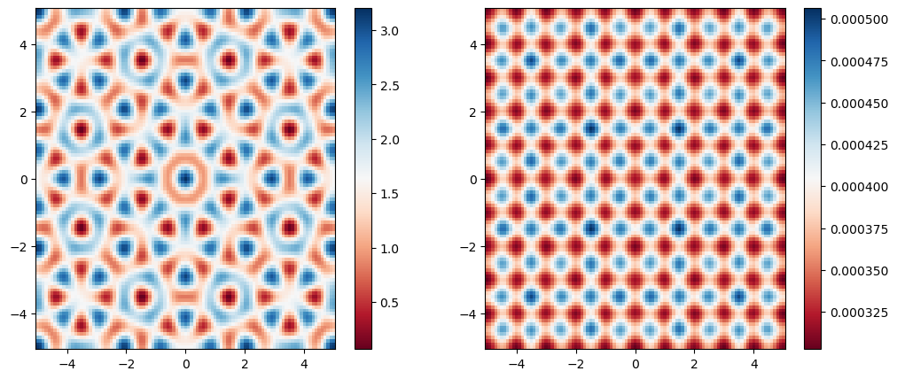
 1V₀ = 0.8
 2L = 50.0
 3Δx² = 0.1
 4N = Int64(div(2L, Δx²))
 5
 6X, Y = meshgrid(LinRange(-L, L, N), LinRange(-L, L, N));
 7V = QC.(X, Y, V₀)
 8ef = eigenfunctionDBCKrylov(V, L, N)
 9
10fig, axes = subplots(nrows=1, ncols=2, figsize=(12, 5))
11im1 = axes[1].pcolormesh(X[450:550,450:550], Y[450:550,450:550], V[450:550,450:550], cmap=:RdBu)
12colorbar(im1, ax=axes[1])
13im2 = axes[2].pcolormesh(X[450:550,450:550], Y[450:550,450:550], ef[450:550,450:550]^2, cmap=:RdBu)
14colorbar(im2, ax=axes[2])
PyObject <matplotlib.colorbar.Colorbar object at 0x000000006E89FF40>
 1# @pyimport matplotlib.animation as anim
 2# using Base64
 3
 4# fig = figure(figsize=(6.2,5))
 5
 6# function make_frame(i)
 7#     V₀ = 0.02*i
 8#     L = 10.0
 9#     N = 150
10
11#     X, Y = meshgrid(LinRange(-L, L, N), LinRange(-L, L, N));
12#     V = QC.(X, Y, V₀)
13#     ef = eigenfunctionDBC(V)
14
15#     pcolormesh(X, Y, ef^2, cmap=:RdBu)
16# end
17
18# withfig(fig) do
19#     myanim = anim.FuncAnimation(fig, make_frame, frames=20, interval=200)
20#     myanim[:save]("test2.mp4", bitrate=-1, extra_args=["-vcodec", "libx264", "-pix_fmt", "yuv420p"])
21# end
22
23# function showanim(filename)
24#     base64_video = base64encode(open(filename))
25#     display("text/html", """<video controls src="data:video/x-m4v;base64,$base64_video">""")
26# end
27# showanim("test2.mp4")