Automatic differentiation of a recursive partition function
This tutorial demonstrates how to compute the energy of a bosonic gas in a harmonic trap using automatic differentiation.
1using ForwardDiff: derivative
2using CairoMakie, ProgressMeter
3using BenchmarkTools
4
5using Pkg; Pkg.status()
Status `/var/home/oameye/Documents/hugo-toha/content/posts/automatic_differentiation/Project.toml`
  [13f3f980] CairoMakie v0.15.3
  [634d3b9d] DrWatson v2.18.0
  [f6369f11] ForwardDiff v1.0.1
  [98b081ad] Literate v2.20.1
  [92933f4c] ProgressMeter v1.10.4
1using InteractiveUtils
2InteractiveUtils.versioninfo()
Julia Version 1.10.10
Commit 95f30e51f41 (2025-06-27 09:51 UTC)
Build Info:
  Official https://julialang.org/ release
Platform Info:
  OS: Linux (x86_64-linux-gnu)
  CPU: 12 × AMD Ryzen 5 5600X 6-Core Processor
  WORD_SIZE: 64
  LIBM: libopenlibm
  LLVM: libLLVM-15.0.7 (ORCJIT, znver3)
Threads: 10 default, 0 interactive, 5 GC (on 12 virtual cores)
Environment:
  JULIA_EDITOR = code
  JULIA_VSCODE_REPL = 1
  JULIA_NUM_THREADS = 10
In statistical mechanics, the partition function is a central quantity that encodes all thermodynamic information of a system. For a bosonic gas in a harmonic trap, we need to compute the energy by differentiating the logarithm of the partition function with respect to the inverse temperature $β$.
The energy of a quantum system is given by: $$ E = -\frac{\partial}{\partial \beta} \ln Z(\beta) $$ where $Z(β)$ is the partition function and $β = 1/(k_B T)$ is the inverse temperature.
Single-Particle Partition Function
The single-particle partition function for a d-dimensional harmonic oscillator: $$ z(\beta, d) = \left(\frac{e^{-\beta/2}}{1-e^{-\beta}}\right)^d $$ This accounts for the zero-point energy $(1/2)ℏω$ and the geometric series from the discrete energy levels $n·ℏω$.
1function z(β, d)
2    return (exp(-0.5*β)/(1-exp(-β)))^d
3end;
Many-Body Partition Function
For N indistinguishable bosons, the partition function is computed recursively. This accounts for the bosonic statistics where multiple particles can occupy the same quantum state. The recursive formula is: $$ Z(N, \beta, d) = \frac{1}{N} \sum_{k=1}^{N} z(k\beta, d) \cdot Z(N-k, \beta, d) $$ with the boundary condition $Z(0, β, d) = 1$.
This recursion arises from the cluster expansion of the grand canonical partition function, accounting for all possible ways to distribute N particles among the available energy levels.
1function Z(N, β, d)
2    if N == 0
3        return 1.0
4    else
5        return (1 / N) * sum(z(k * β, d) * Z(N - k, β, d) for k in 1:N)
6    end
7end;
Energy Calculation via Automatic Differentiation
The energy is computed as the negative logarithmic derivative of the partition function: $$ E = -\frac{\partial}{\partial \beta} \ln Z(\beta) $$
We implement two different approaches:
- Bosonic: Uses the full many-body partition function Z(N, β, d)
- Boltzmann: Uses the classical approximation z(β, d)^N (non-interacting)
The automatic differentiation (via ForwardDiff) computes the derivative analytically without numerical approximation, making it both accurate and efficient.
1function energy(N::Int64, β::Float64, d::Int64; type::Symbol = :boson)
2    if type == :boson
3        return -derivative(x -> log(Z(N, x, d)), β)
4    else type == :boltzmannon
5        return -derivative(x -> log(z(x, d)^N), β)
6    end
7end;
Numerical Experiment
We now compute the energy for different numbers of particles N and different inverse temperatures β. This allows us to study:
- How the energy depends on temperature $(β = 1/T)$
- How quantum statistics affect the energy for different particle numbers
- The transition from quantum to classical behavior
Parameter Space
- N: Number of particles $[1, 5, 10, 20]$
- β: Inverse temperature range $[1, 10]$ (corresponds to $T ∈ [0.1, 1]$)
- d: Dimensionality = 1 (1D harmonic oscillator)
1range2d = Iterators.product([1, 5, 10, 20], 1:0.1:10)
2mat = @showprogress map(range2d) do (N, β)
3    energy(N, β, 1)
4end
4×91 Matrix{Float64}:
  1.08198   0.998961   0.931013   0.874631   0.827311   0.787217   0.75297   0.723516   0.698034   0.675874   0.656518   0.639545   0.62461   0.611431   0.599769   0.589425   0.580233   0.572048   0.564747   0.558227   0.552396   0.547174   0.542494   0.538296   0.534525   0.531138   0.528091   0.52535   0.522883   0.52066   0.518657   0.516852   0.515224   0.513755   0.51243   0.511234   0.510154   0.509179   0.508298   0.507502   0.506784   0.506134   0.505547   0.505017   0.504537   0.504104   0.503712   0.503357   0.503037   0.502747   0.502485   0.502248   0.502034   0.50184   0.501664   0.501506   0.501362   0.501232   0.501115   0.501009   0.500913   0.500826   0.500747   0.500676   0.500612   0.500553   0.500501   0.500453   0.50041   0.500371   0.500336   0.500304   0.500275   0.500249   0.500225   0.500204   0.500184   0.500167   0.500151   0.500136   0.500123   0.500112   0.500101   0.500091   0.500083   0.500075   0.500068   0.500061   0.500055   0.50005   0.500045
  3.66075   3.43331    3.26044    3.12679    3.02189    2.93842    2.87119   2.81645    2.77143    2.73409    2.70286    2.67655    2.65424   2.63522    2.61891    2.60485    2.59269    2.58212    2.5729     2.56484    2.55776    2.55153    2.54604    2.54118    2.53687    2.53305    2.52965    2.52662   2.52392    2.52151   2.51935    2.51742    2.51568    2.51413    2.51274   2.51148    2.51036    2.50935    2.50844    2.50761    2.50688    2.50621    2.50561    2.50507    2.50458    2.50414    2.50374    2.50338    2.50306    2.50276    2.5025     2.50226    2.50204    2.50185   2.50167    2.50151    2.50137    2.50124    2.50112    2.50101    2.50091    2.50083    2.50075    2.50068    2.50061    2.50055    2.5005     2.50045    2.50041   2.50037    2.50034    2.5003     2.50027    2.50025    2.50023    2.5002     2.50018    2.50017    2.50015    2.50014    2.50012    2.50011    2.5001     2.50009    2.50008    2.50007    2.50007    2.50006    2.50006    2.50005   2.50005
  6.18629   5.94648    5.76729    5.63038    5.52377    5.43941    5.37172   5.31673    5.27158    5.23417    5.2029     5.17657    5.15426   5.13523    5.11891    5.10486    5.09269    5.08212    5.0729     5.06484    5.05776    5.05153    5.04604    5.04118    5.03687    5.03305    5.02965    5.02662   5.02392    5.02151   5.01935    5.01742    5.01568    5.01413    5.01274   5.01148    5.01036    5.00935    5.00844    5.00761    5.00688    5.00621    5.00561    5.00507    5.00458    5.00414    5.00374    5.00338    5.00306    5.00276    5.0025     5.00226    5.00204    5.00185   5.00167    5.00151    5.00137    5.00124    5.00112    5.00101    5.00091    5.00083    5.00075    5.00068    5.00061    5.00055    5.0005     5.00045    5.00041   5.00037    5.00034    5.0003     5.00027    5.00025    5.00023    5.0002     5.00018    5.00017    5.00015    5.00014    5.00012    5.00011    5.0001     5.00009    5.00008    5.00007    5.00007    5.00006    5.00006    5.00005   5.00005
 11.1866   10.9466    10.7673    10.6304    10.5238    10.4394    10.3717   10.3167    10.2716    10.2342    10.2029    10.1766    10.1543   10.1352    10.1189    10.1049    10.0927    10.0821    10.0729    10.0648    10.0578    10.0515    10.046     10.0412    10.0369    10.033     10.0296    10.0266   10.0239    10.0215   10.0193    10.0174    10.0157    10.0141    10.0127   10.0115    10.0104    10.0093    10.0084    10.0076    10.0069    10.0062    10.0056    10.0051    10.0046    10.0041    10.0037    10.0034    10.0031    10.0028    10.0025    10.0023    10.002     10.0018   10.0017    10.0015    10.0014    10.0012    10.0011    10.001     10.0009    10.0008    10.0007    10.0007    10.0006    10.0006    10.0005    10.0005    10.0004   10.0004    10.0003    10.0003    10.0003    10.0002    10.0002    10.0002    10.0002    10.0002    10.0002    10.0001    10.0001    10.0001    10.0001    10.0001    10.0001    10.0001    10.0001    10.0001    10.0001    10.0001   10.0
We plot the energy as a function of inverse temperature β for different particle numbers N. The log-log scale reveals the power-law behavior in different temperature regimes:
- High temperature (small β): Classical behavior E ∝ T
- Low temperature (large β): Quantum behavior dominated by zero-point energy
Each curve represents a different particle number, showing how bosonic statistics modify the energy compared to the classical case.
 1fig = Figure(size = (400, 250), fontsize = 7)
 2ax = Axis(fig[1, 1],
 3          xscale = log10,
 4          yscale = log10,
 5          xlabel = "Inverse Temperature β",
 6          ylabel = "Energy E",
 7          title = "Energy of Bosonic Gas in Harmonic Trap")
 8
 9for (i, N) in enumerate([1, 5, 10, 20])
10    row = mat[i, :]
11    lines!(ax, 1:0.1:10, row, label = "N = $N")
12end
13Legend(fig[1,2], ax)
14fig
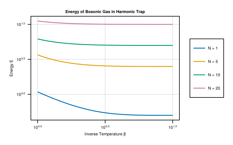
The results show several important features:
- Zero-point energy: Even at $T → 0 (β → ∞)$, the energy remains finite due to quantum fluctuations
- Bosonic enhancement: Higher particle numbers show deviations from classical behavior due to quantum statistics
- Temperature scaling: The energy follows different power laws in different temperature regimes
Version Information
1using InteractiveUtils
2InteractiveUtils.versioninfo()
1using Pkg
2Pkg.status()
This page was generated using Literate.jl.